概述
Mini-Batch Gradient Descent是介于batch gradient descent(BGD)和stochastic gradient descent(SGD)之间的一种线性回归优化算法,它是将数据分为多个小的数据集(batches),每个数据集具有大致相同的点数,然后在每个数据集中应用Absolute Trick或者是Square Trick算法,来更新回归系数。
它的运算速度比BSD快,比SGD慢;精度比BSD低,比SGD高。
代码
1 | import numpy as np |
结果
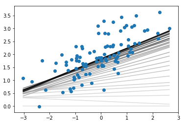
在结果中,颜色最浅的是最开始的回归线,最深的则为最终的回归线。
详解
理论知识参见Linear Regression 总结,这里只对代码中出现的新函数或新用法进行讲解。
numpy.matmul(a,b)
该函数用来计算两个arrays的乘积。
需要注意的是,由于a和b维度的不同,会使得函数的结果计算方式不同,一共三种:
如果a和b都是2维的,则做普通矩阵乘法
1
2
3
a = [[1, 0], [0, 1]]
b = [[4, 1], [2, 2]]
np.matmul(a, b)1
2
3out:
array([[4, 1],
[2, 2]])如果a和b中有一个是大于2维的,则会将其理解为多个矩阵stack后的结果,进行计算时也会进行相应的拆分运算
1
2
3a = np.arange(2*2*4).reshape((2,2,4))
b = np.arange(2*2*4).reshape((2,4,2))
np.matmul(a,b).shape1
2out:
(2, 2, 2)a被理解为2个2x4矩阵的stack
1
2
3
4
5array([[[ 0, 1, 2, 3],
[ 4, 5, 6, 7]],
[[ 8, 9, 10, 11],
[12, 13, 14, 15]]])b被理解为2个4x2矩阵的stack
1
2
3
4
5
6
7
8
9array([[[ 0, 1],
[ 2, 3],
[ 4, 5],
[ 6, 7]],
[[ 8, 9],
[10, 11],
[12, 13],
[14, 15]]])np.matmul(a,b)会将a中的两个矩阵与b中的两个矩阵对应相乘,每对相乘的结果都是一个2x2的矩阵,所以结果就是一个2x2x2的矩阵。如果a或b有一个是一维的,那么就会为该一维数组补充1列或1行,进而提升为二维矩阵,然后用非补充行或列去和另外一个二维矩阵进行运算,得到的结果再将补充的1去掉。(这个是最难理解的,可以多测试下,用代码结果理解)
1
2
3
a = [[1, 0], [0, 1]]
b = [1, 2]
np.matmul(a, b)1
2out:
array([1, 2])a是一个2x2的矩阵,b是一个shape为(2,)的一维数组,那么matmul的计算步骤如下:
- 计算中,矩阵a在前,数组b在后,所以需要让a的列数与升维之后b矩阵的行数相等
- 所以,升维后b矩阵的shape应为(2,1),这个1添加到了列上
- 进行矩阵乘法计算,得到shape为(2,1),这时候再将这个1去掉
- 最终结果的shape为(2,),变为一维数组
我们试着将a与b的顺序对调,看一下matmul是怎么计算的:
- 对调后,数组b在前,矩阵a在后,需要将升维后b矩阵的列数与矩阵a的行数相等
- 所以,升维后b矩阵的shape应该为(1,2),这个1添加到了行上
- 进行矩阵乘法,得到的shape为(1,2),将这个1去掉
- 最终结果的shape为(2,),变为一维数组
numpy.hstack()
我们先来看看numpy.stack()函数。
- 函数用法为:numpy.stack(arrays,axis = 0)
- 第一个参数为arrays,可以输入多维数组或者列表,也可以输入由多个一维数组或列表组成的元组
- 第二个参数为axis,输入数字,决定了按照arrays的哪个维度进行stack。比如说,输入的arrays的shape为(3,4,3),那么axis = 0/1/2就分别对应arrays的组/行/列。
这个函数中的axis有些抽象,我们看具体示例:
- 定义了一个列表
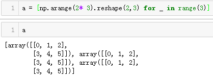
结果的排版有点问题,为了方便后面对照,把结果对齐如下:
1 | [ |
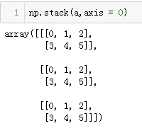
axis = 0,则按照第0个维度
组进行堆叠,即: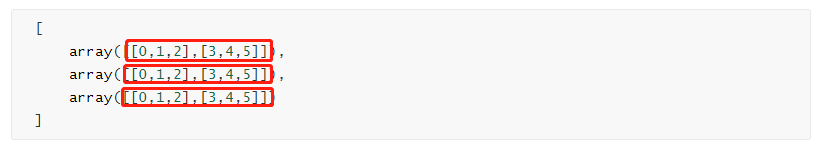
结果为:
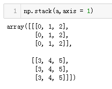
axis = 1,则按照第1个维度
行进行堆叠,即: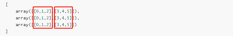
结果为:
axis = 2,则按照第二个维度
列进行堆叠,即: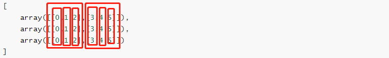
结果为:

这个基本很少用到。
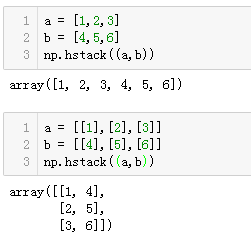
**numpy.hstack()**函数就是horizontal(水平)方向的堆叠,示例:
**numpy.vstack()**函数就是在垂直方向堆叠。
ndarray的切片
一维ndarray的切片方式和list无异,这里主要讲一下二维矩阵的切片方法。
- 矩阵切片
1 | a = np.arange(4*4).reshape(4,4) |
1 | out: |
1 | a[:,:-1] |
1 | out: |
这里可以看出,我们筛选了a矩阵中前三列的所有行,这是如何实现的呢?
切片的第一个元素:表示的是选择所有行,第二个元素:-1表示的是从第0列至最后一列(不包含),所以结果如上所示。
再看一个例子:
1 | a[1:3,:] |
1 | out: |
筛选的是第2-3行的所有列。
- 一个常用的切片
以列的形式获取最后一列数据:
1 | a[:,3:] |
1 | out: |
以一维数组的形式获取最后一列数据:
1 | a[:,-1] |
1 | out: |
上面两种方法经常会用到,前者的shape为(4,1),后者为(4,)。
matplotlib相关
color
代码中涉及到的语句为:
1
color = [1 - 0.92 ** counter for _ in range(3)]
matplotlib中的color可以输入RGB格式,即[R,G,B],这里值得注意的是它们的取值范围都在0到1之间,其中[0,0,0]为黑色,[1,1,1]为白色。
在如上语句中,列表由三个相等的数值元素组成,保证了颜色为白-灰-黑,数值随着counter的减小,由1趋近于0,反映在可视化上就是颜色由白逐渐变黑。
这真是一个画渐变过程的好方法呀!!!
plot([x_1,x_2],[y_1,y_2])
这里就是两点式绘图,根据点(x_1,y_1)和点(x_2,y_2)画一条直线。
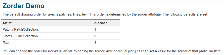
zorder
也就是z-order,类似于PS里面的图层顺序,下面的图层会被上面的图层遮挡。
参考Zorder Demo中队zorder的介绍,可以知道,zorder越大,图层越靠上,所以在上面的代码中,我们在scatter中设定zorder为3,也就是最上层,这样就可以保证渐变的回归线不会压在散点图上面了。